Mathematics
This portfolio illustrates how I approach problems as a mathematician, combining intuition, rigor, and practical data analysis. I use Principal Component Analysis (PCA) as an example, highlighting both its application and its deeper connection to linear algebra via Singular Value Decomposition (SVD).
PCA is often described as an unsupervised learning technique because it identifies patterns in data without predefined labels. In practice, it is a tool for dimensionality reduction, noise filtering, and identifying dominant modes of variability. PCA is also a special case of SVD, which underpins many data-science methods from compression to natural language processing. Understanding this connection provides insight into both the mechanics and the intuition of PCA.
Dataset & Set Up
I used NOAA's Extended Reconstructed Sea Surface Temperature (ERSST) dataset, which reports monthly global sea surface temperature (SST) on a 2° latitude × 1° longitude grid from 1854 to the present. The dataset can be accessed in Python using xarray:
iri_url = "http://iridl.ldeo.columbia.edu/SOURCES/.NOAA/.NCDC/.ERSST/.version5/.sst/"
T_convert = "T/[(days)(since)(1960-01-01)]sconcat/streamgridunitconvert/"
url = iri_url + T_convert + "dods"

ds = xr.open_dataset(url)
For this exploration, I focused on the equatorial Pacific (30°S–30°N, 120°E–60°W) between 1854 and 2024.
At full resolution, this region contains roughly 2,800 spatial grid points and about 2,000 monthly observations, forming a dataset with 5.6 million individual temperature values. Working directly in such a high-dimensional space is inefficient as the data are highly correlated in both space and time. Neighboring grid points often vary together, and many patterns repeat seasonally or interannually. This redundancy makes PCA an ideal tool. By finding a small set of orthogonal directions that capture most of the variance, PCA lets us describe the essential behavior of the system with far fewer dimensions. In other words, it replaces 2,800 spatial variables with a few modes that still explain most of the observed variability.
To prepare the data for PCA, I reshaped the SST field into a two-dimensional matrix X ∈ ℝn×p, where each row represents a month and each column a spatial location. Each column was standardized to have mean 0 and variance 1, so the entries represent temperature variation from mean at each location over time.
The dominant pattern of seasonality is immediately apparent in Figure 1. Less obvious but still strong is the El Niño Southern Oscillation (the fluctuations in sea surface temperature in the equatorial region). These dominant modes should emerge in the leading principal components, illustrating that PCA identifies the key structures in the dataset, whether they are obvious physical phenomena (as they are here) or subtle statistical modes.
Figure 1: Animation ofstandardized sea surface temperature showing dominant seasonal patterns
PCA Intuition
Given a data matrix X ∈ ℝn×p, where n is the number of samples and p the number of variables, PCA finds a new coordinate system where the axes are ordered by how much of the dataset's variance they explain. Formally,
P = XW
where the columns of W are the principal axes, i.e. the eigenvectors of the covariance matrix of X. Each column of P (the principal components) represents the projection of the data onto one of these axes. The first component captures the direction of maximum variance, the second captures the next most variance subject to being orthogonal to the first, and so on.
Because the majority of the variance tends to be concentrated along just a few of these directions, the original dataset can often be reconstructed accurately using only the first m components (where m ≪ s):
X ≈ PmWm⊤
This low-rank approximation is one way in which PCA valuable. It reduces the number of variables needed to describe a system from thousands to just a handful while retaining most of the meaningful structure. In many high-dimensional datasets, this is what makes analysis and modeling computationally feasible without sacrificing interpretability.
Implementation and Visualization
PCA can easily be implemented using scikit-learn. As we expected, the first principal component captures seasonality while the second isolates ENSO. We can visualize these patterns by projecting the data onto a single principal axis. Figure 2 shows the seasonality, captured by the opposing northern and southern Pacific temperature patterns. Figure 3 highlights the central and eastern equatorial Pacific, corresponding to El Niño and La Niña events. The magnitude of these projections correlates with known event intensities (e.g., 2010–2011 La Niña, 2015–2016 El Niño).
Figure 2: First principal component capturing seasonal temperature patterns
Figure 3: Second principal component highlighting ENSO
Reconstructing SST
PCA enables low-dimension reconstruction of the data with controllable accuracy. Suppose we want to model SST with 95% accuracy. We can see how many dimensions are necessary to achieve this. Using scikit-learn's PCA implementation, the cumulative explained variance (Figure 4) shows that 14 principal components capture 95% of the total variance. This is an enormous compression from the original 2,800 spatial dimensions, reducing the total data size to roughly 0.5% of the original.
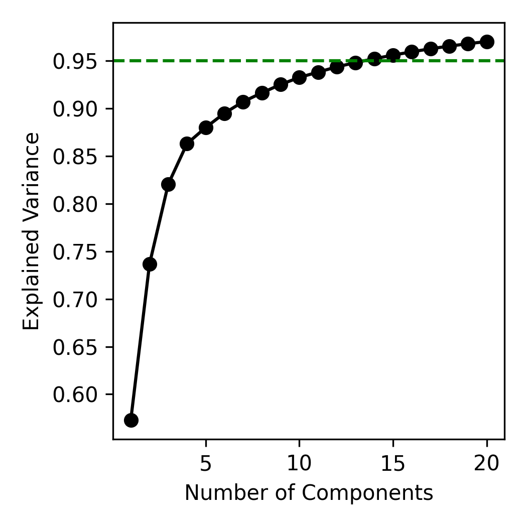
Figure 4: Explained variance as a function of number of components
Figure 5 shows the reconstructed SST from these 14 components compared to the original data. The two are nearly indistinguishable. The slight differences correspond mostly to small-scale, high-frequency noise that contributes little to the system's total variance.
Figure 5: Reconstructed SST using 14 components
PCA and SVD
This section is a condensed version of a previous blog post.
Principal Component Analysis (PCA) and Singular Value Decomposition (SVD) are often presented as separate concepts, when in fact PCA is just a special case of SVD. Typically, PCA is used and presented as a tool that seeks orthogonal directions (principal axes) that capture maximal variance in a dataset, while SVD decomposes a matrix into orthogonal transformations and a diagonal scaling. Understanding how these two formulations align clarifies both the mechanics and intuition behind PCA.
In the traditional derivation, PCA begins with the covariance matrix:
C = (1/(n−1)) X⊤X
where X is a centered data matrix with n samples and p variables. The eigenvectors of C define the principal axes, and the corresponding eigenvalues quantify the variance along each axis. Projecting the data onto these eigenvectors yields the principal components. This variance-based route frames PCA as a statistical tool for simplifying high-dimensional data while retaining its most informative patterns.
SVD generalizes the same idea geometrically. Any real matrix X can be factored as:
X = USV⊤
where U and V are orthogonal matrices and S is diagonal with nonnegative singular values. The right singular vectors in V correspond exactly to the eigenvectors of the covariance matrix C, that is, the principal axes, and the left singular vectors U (scaled by S) correspond to the principal components. The singular values relate to the eigenvalues by:
λi = si2 / (n−1)
Geometrically, SVD expresses X as a rotation, followed by axis-aligned scaling, and another rotation, providing a clean visualization of how PCA "rotates" the data to align with its directions of greatest variance.
This equivalence reveals two complementary views of PCA: the covariance-based perspective explains what PCA achieves, identifying directions of maximal variance, while the SVD perspective explains how it achieves it, through orthogonal rotations and scalings that diagonalize the covariance structure. Seeing PCA as a direct application of SVD unifies its statistical and geometric interpretations, and underscores that PCA is not just a variance-maximizing heuristic, but a precise linear-algebraic transformation that exposes the intrinsic structure of data.
Code Availability
The code for this work is available on my GitHub.